What Dynamic Simulation Does?

I hope you’ve got your preferred drink in hand ☕️🫖💧

📬 📰 Saturday editions - for having more time to read during the weekend! Let’s experiment for a few weeks. Let me know if this is not a convenient day (❓).

Last week, we solved a puzzling question: which tank empties first? And while at the beginning one could think they would empty in the same amount of time, we reflected on how things would look like “a small amount of time later”… and it became clear that one would definitely empty faster than the other.

At this point, we touched about the need for Dynamic Simulation.

Today, let’s dig into what dynamic simulation is.

Useless note: One could argue that this should have been one of the first posts, and as it is the number 10, it is indeed just the second somehow… (“There are 10 types of people: those who know how to count in binary and those who don’t”)

The status quo

Let’s take another example. I love bicycles so let’s talk about bikes. 🚲

Similar to the runner’s case, we might want to calculate the force we have to push on the pedals to keep a cruise speed of 20km/h on a flat road or going uphill. We can study with or without a headwind. (And if you are in the UK or US or other non-SI unit country 😉, just change km/h for mph and you’ll just have to go about 1.6 times faster. Good luck! 😉)

See how we naturally wanted to calculate THE force? For each case, we are looking at an equilibrium: the speed is one value, and so the force is one value too. Sure, there are boundary conditions, namely the slope and the wind. And we can create test cases making these boundary conditions change. For each, we’ll get the value of the force.

And for each case, there is only one force because we are at equilibrium - here constant speed. This is a steady-state analysis. For the tanks, imagine the tap would be closed: the pressure at the bottom would be constant and there would be no flow to change this “status quo”. But what happens if we open the tap?

It’s about the journey

You know the quotes that go something like:

it is not about the destination, it’s about the journey.

(There are many quotes that sound similar so this one might be slightly different to the one you know, and it is hard to provide the credit to someone specific. Anyway…)

Dynamic simulation is like that: less about the (steady-state) destination, and more about the journey.

So you know an initial “state”. (We’ll talk about what a state really is later.) And this state is not at equilibrium - not steady. So the game of dynamic simulation is to “predict” how the system state will evolve over time. Until… the desired time (or a steady-state!).

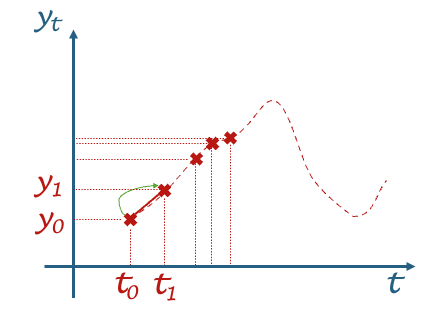
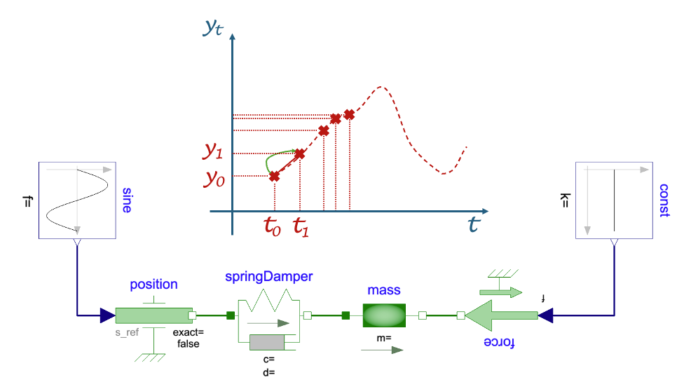
Dynamic simulation is about computing the trajectory of the states

The time t_0 represents an initial time and we know the value of the state y at this time - hence y_0. We want to find out y_1 at time t_1 and so on. And you notice how the times are not necessarily equally spaced? This is for another day, yet just keep in mind that the steps we take are not necessarily equally spaced.

But eh, the dashed line is the solution, let’s just use it, no? Well of course, we don’t know it! I just put it there for you to see that the goal is to predict the points (❌) on the line. And in between the points? We can interpolate, with the right level of smoothing.

So how do we make sure that we “predict” the right values? Well, there is not much luck into this: we don’t really predict but compute. And we compute based on our model - as we saw over the last 10 posts!

From equations to solutions

It is hard to talk about simulation without really showing an equation. Let me try to keep it to the minimal.

Dynamic systems involve dynamics… and dynamics are modeled with differential equations. Basically something like:

y_dot = f(y,u,t)

And y_dot is the time derivative of y. But what does that mean? The time derivative of a variable is the rate of change of this variable over time. It basically tells you in which direction and at which “pace” it will change its value. u are potential inputs (e.g. the speed of the wind or the ground slope)

So if we know the speed v of our runner and we keep in mind that the speed is the derivative of the position x, then we can - knowing the initial position of the runner and its speed - compute its new position after a given amount of time (assuming the speed does not change in this amount of time).

So now we have the question: do we know the new speed? Well, actually, if we have the equation v = f(x , u, t) and we know x, (potentially u,) and t then we can compute v!

So now we just need to get the new value of x at the next time step. And so it goes.

You are hiding something!

I kind of hide something here… how do you compute x knowing v? Well that is what a solver does. I don’t want to enter today into that topic because it is already quite a long theoretical article… but the simplest (not the best) solver is Forward Euler and I explain it here if you are impatient. 😊

And the right question to ask next is whether we cannot just solve the differential equation analytically instead of using a solver? Yes, in theory. It however gets really complex really fast because we usually have many variables and the equations are all but simple. So in practice, it is often impossible. Solvers are key to our simulations.

An example to wrap things up

One of the first example I learned was a “quarter of a vehicle”. It basically means that you take a car, you cut it in 4 and look at a quarter. It is a fair thing to do if you assume the weight distribution to be equally spread over the four wheels. And we just look at the vertical displacement.

So you have a very simple model that looks like a typical oscillator: a mass (quarter of the car mass) on which applies gravity (here the constant force), a spring-damper for the suspension and the floor that is slightly moving because it is not perfectly flat.

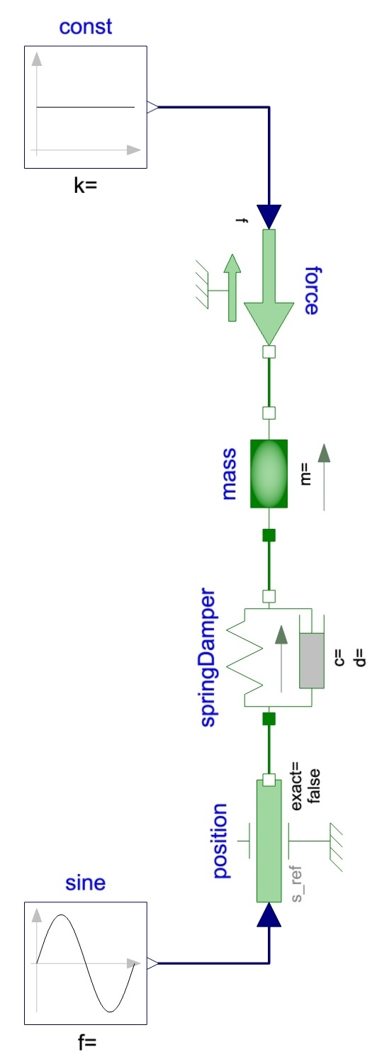
Assume the car is stopped. The floor won’t be moving with respect to the car… hopefully. We can see by simulating, how much the car will “sink” on its suspension and which steady-state it will reach.

Now if we start driving, we will have the height of the floor constantly changing and that induces a compression on the spring and some dissipation from the damper. A resulting force will be applied to the mass that will be combined with the gravity… I might have lost you here. If so, go to the next paragraph, it is OK. If not, let’s continue: Newton told us that the sum of forces - over a constant mass (taking shortcuts here) - equals the mass multiplied by the acceleration. Acceleration! We get the new acceleration and that is the derivative of the speed, so we can use the solver to compute it! And from the speed, the position! Tadaaaam! And we can just go to the next step and repeat.

Basically, the model you build will have the equations behind to express the relations between the states of your system and their derivatives. And so you’ll be able to compute these and let the solver tell you what the next states are.

And hopefully, the mass (on which you might be sitting - the car - but not while reading this!) might not oscillate too much!

The END for today

Enough for today. This was an abstract one and I hope it’s OK. I had to cover the process.

Next time, we will go into something more applied. I initially wanted to cover what solvers do, but unless you say it in comments, I will wait a bit so we get some actual modeling going on first.

Break is over, go back to what you were doing.

Clem

Next ->